Posts

|| Dyanamic Stacked Chart ||
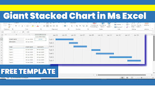
Image
Make a Gantt Chart in Excel To create a stacked chart in Microsoft Excel, follow these steps: 1. Select the data you want to chart, including the categories and values. 2. Go to the "Insert" tab in the ribbon. 3. Click on the "Column" or "Bar" chart button (depending on your preference). 4. Select the "Stacked" chart subtype. 5. Choose the chart layout and formatting options as desired. 6. Click "OK" to create the chart. Tips: - Make sure your data is organized with categories in one column and corresponding values in another. - Use the "Series" option to select which columns to include in the stack. - Use the "Axis Label" option to customize the labels on the x and y axes. - Use the "Legend" option to customize the chart legend. Here's a more detailed step-by-step guide: 1. Select the data range (A1:B5, for example). 2. Go to the "Insert" tab. 3. Click on "Column" or "Bar"...

AI with Excel-: Everything You Need To Know

Image
  Building a data presentation within an Excel   spreadsheet   can be tricky if you are not a Microsoft Excel power user that understands each Excel formula inside out. While several features within Microsoft Excel can help bring your tabular data set to life, it is hard to find out what each is and even harder to remember them! It is no surprise that many people find  Microsoft Excel  much more challenging to use than Microsoft PowerPoint or Excel. But it doesn't have to be. Through machine learning algorithms, even Excel novices can undertake data science and build detailed datasets that help them achieve their objectives.  If you're a visual learner, you can also watch  the video below  and subscribe for the best spreadsheet tips online.  Machine learning can replace manual data input.  Manually inputting data into a  spreadsheet   is not fun for anyone. It is an incredibly time-consuming process that takes plenty of human r...

xlookup multiple criteria By Hamid Shigri

Image
Download by this Below Link Xlookup Multiple criteria

Consolidate data in Excel and merge multiple sheets into one worksheet

Image
 The tutorial demonstrates different ways to combine sheets in Excel depending on what result you are after - consolidate data from multiple worksheets, combine several sheets by copying their data, or merge two Excel spreadsheets into one by the key column. Today we will tackle a problem that many Excel users are struggling with daily - how to merge multiple Excel sheets into one without copying and pasting. The tutorial covers two most common scenarios: consolidating numeric data (sum, count, etc.) and merging sheets (i.e. copying data from multiple worksheets into one). Consolidate data from multiple worksheets in a single worksheet The quickest way to consolidate data in Excel (located in one workbook or multiple workbooks) is by using the built-in Excel Consolidate feature. Let's consider the following example. Supposing you have a number of reports from your company regional offices and you want to consolidate those figures into a master worksheet so that you have one summary...

How to Use VLOOKUP in Excel? A Step-by-Step Guide

Image
  Introduction About VlookUp VLOOKUP stands for Vertical Lookup. As the name specifies, VLOOKUP is a built-in Excel function that helps you look for a specified value by searching for it vertically across the sheet. Excel provides an extensive range of functions that makes it easier to work with data. VLOOKUP in Excel is one such function. VLOOKUP works as a search function by looking for specific data vertically across a table or spreadsheet. Let’s go ahead and understand what exactly VLOOKUP in Excel is. What is VLOOKUP in Excel? VLOOKUP stands for Vertical Lookup. As the name specifies, VLOOKUP is a built-in Excel function that helps you look for a specified value by searching for it vertically across the sheet. VLOOKUP in Excel may sound complicated, but you will find out that it is a very easy and useful tool once you try it. Look at the example below to understand VLOOKUP . The VLOOKUP formula below looks for a Company name with Company ID 3. In the next section, you will...

What Is Excel Index?

Image
Excel Index An index column is also added to an Excel worksheet when you load it. To open a query, locate one previously loaded from the Power Query Editor, select a cell in the data, and then select Query > Edit. For more information see Create, load, or edit a query in Excel (Power Query). Select Add Column > Index Column. Index Formula.. =INDEX(array, row_num, [col_num]) The function uses the following arguments: Array (required argument) – This is the specified array or range of cells. Row_num (required argument) – Denotes the row number of the specified array. Some Examples With Images